metrology frame and multi-axis dynamic error analysis for subatomic nano-positioning flexure stage
· manufacturing, research
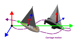
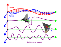
flexure stages are understood to be the pinnacle of precision motion control. however, nothing is truly perfect. although flexures constrain motion incredibly well into the designed axis, parasitic motion is can still be evident. obviously this isnt an issue in most cases, but understanding these limitations is important for the furthering of ultra precision motion control.
low frequency error calibration is what is usually tested, as it is the easiest to implement. things like straightness and angular errors. however in practice these stages get used dynamically, driven by a piezoelectric actuated high-speed control system in this case, at a bandwidth that would not typically be analyzed. this project was about building a testbed to capture the full 6-DOF motion of a flexure carriage in real time at this high bandwidth.
the testing stage
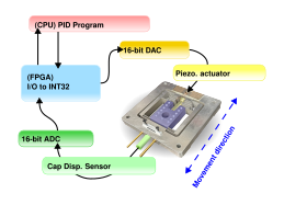
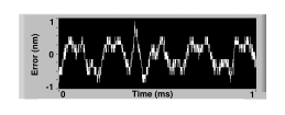
the stage under test is a double-compound rectilinear flexure driven by a piezoelectric actuator. its position is measured by a capacitive displacement sensor in a closed loop running on an FPGA at up to 50 ksps. the PID controller holds positioning error within about 1 nm of the setpoint in a non-controlled lab environment.
measuring the errors
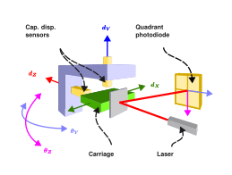
the metrology system measures five error channels, two being rectilinear (\(y\) and \(z\) straightness) and three angular (\(\theta_x\), \(\theta_y\), \(\theta_z\)). the sixth DOF, position along the drive axis (\(x\)), comes from the stage's own capacitive sensor.
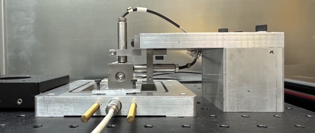
rectilinear errors are captured with lion precision capacitive displacement sensors mounted to a metrology frame. after dynamic simulation analysis the stage was found to be rigid enough to not have any natural frequencies below 1,000 Hz, so this system was deemed sufficiently rigid for this application as a part that does not move.
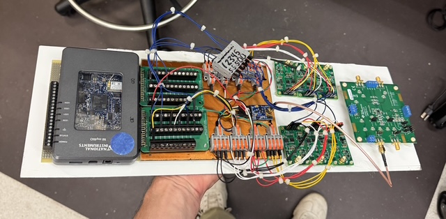
the sensors look at the faces of a gage block sitting on top of the carriage. resolution is limited by the 16-bit ADC (AD5541A), which works out to about 0.18 nm, verified against our agilent machine tool metrology interferometer.
angular measurement via optical lever
angular errors are measured with a pair of laser-quadrant photodiodes. a laser beam reflects off a steering mirror on the gage block and hits a quadrant photodiode some distance away. the intensity distribution across the four quadrants gives you the angular displacement of the mirror. the long lever arm between mirror and detector makes really small rotations produce measurable spot shifts. a second photodiode on an orthogonal axis captures the remaining angular DOF.
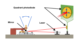
the nice thing about this setup is that angular resolution scales with lever arm length, so you can trade off range for resolution just by moving the photodiode closer or further from the mirror. no hardware changes needed. obviously this is assuming beam quality stays uniform.
reconstructing 6-DOF motion
this is where the math gets interesting. the traditional approach for combining angular measurements into a rotation is euler angles, but euler angles are sequence-dependent and at the sub-microradian scale the ordering artifacts are comparable to the signals you're trying to measure. all we get here is the sum of multiple rotations, so you can instead just use that resulting position to map rotation.
the displacement of the two laser-quadrant photodiodes each provide two components of a direction vector. call these measurement vectors \(\mathbf{A}\) and \(\mathbf{B}\). each photodiode gives you two of the three spatial components:
\[ \theta_X = \tan^{-1}\left(\frac{Y_b}{L_2}\right), \quad \theta_Z = \tan^{-1}\left(\frac{Y_a}{L_1}\right), \quad \theta_{Y} = \frac{1}{2}\left[\tan^{-1}\left(\frac{Z_A}{L_1}\right) + \tan^{-1}\left(\frac{X_b}{L_2}\right)\right] \]but rather than extracting angles, the raw photodiode readings are corrected for rectilinear carriage motion (subtracting out the straightness deviations) and then used directly to construct an orthonormal basis:
\[ \hat{\mathbf{A}} = \frac{\mathbf{A}'}{\lVert \mathbf{A}' \rVert}, \quad \hat{\mathbf{B}} = \frac{\mathbf{B}'}{\lVert \mathbf{B}' \rVert}, \quad \hat{\mathbf{C}} = \frac{\mathbf{A}' \times \mathbf{B}'}{\lVert \mathbf{A}' \times \mathbf{B}' \rVert} \]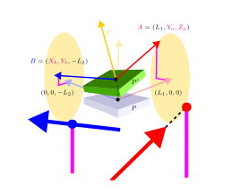
these three basis vectors plus the rectilinear displacement data form a homogeneous transformation matrix:
\[ P' = \begin{bmatrix} | & | & | & d_X \\ \hat{A} & \hat{B} & \hat{C} & d_Y \\ | & | & | & d_Z \\ 0 & 0 & 0 & 1 \end{bmatrix} \begin{bmatrix} P_X \\ P_Y \\ P_Z \\ 1 \end{bmatrix} \]this maps any point on the carriage from its nominal position to its actual position at each discrete time step. the result is a full 6-DOF trajectory for every point on the carriage, at whatever sample rate the DAQ can sustain. from there you can do frequency decomposition per axis, dynamic mode decomposition, modeling, or just look at the trajectory directly.
initial testing
to test i did a sweep from 0 to 2 kHz and looked at the frequency domain data from all 3 axes (spectrogram, psds, and frfs). this data is here: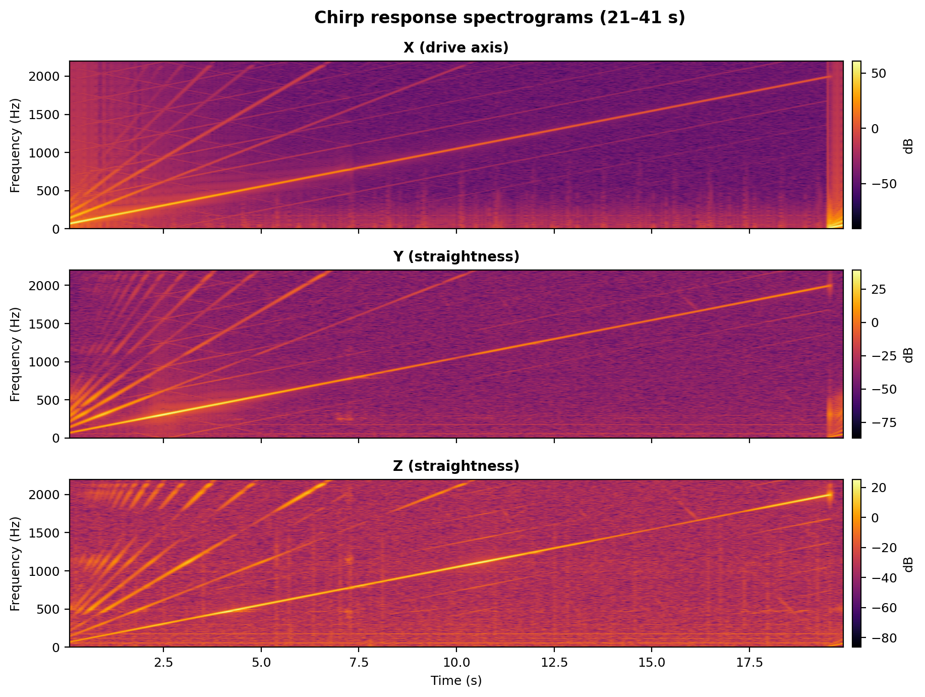
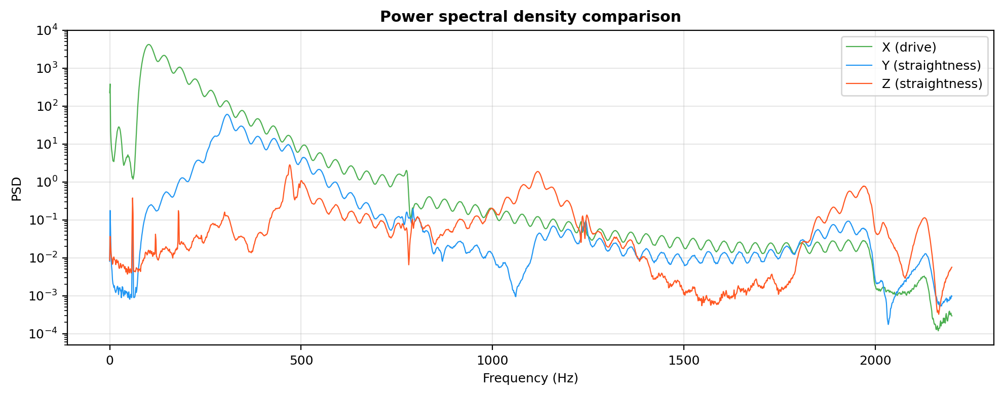
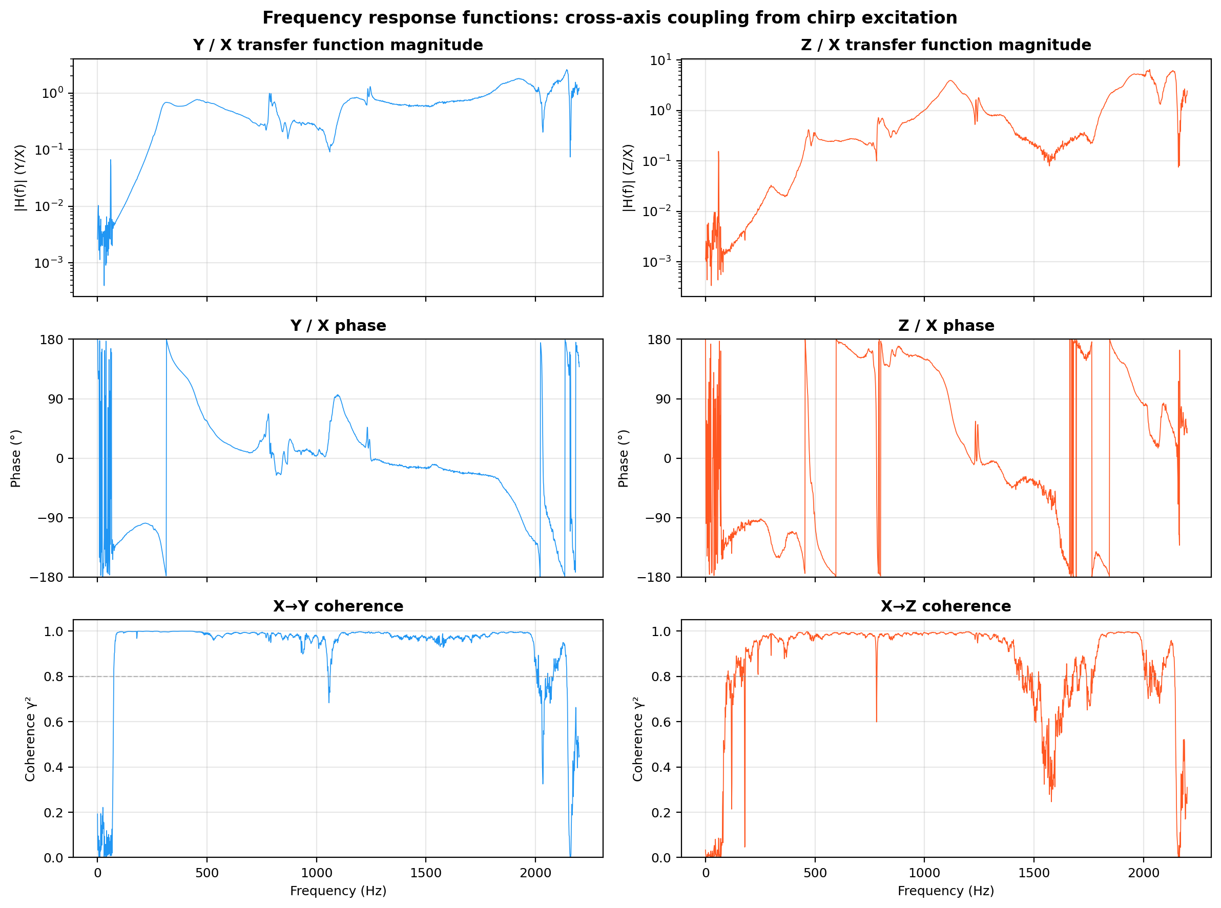
there are some interesting harmonics that show up on all of the axes. this is likely due to the input not exactly equaling the end movement. the chirp signal was driven by a liquid instruments moku:go. this says that it can go up to 20 MHz on the outputs, so i am assuming the input sine wave is quite clean. the analysis assumes that the stage is moving in a perfect sine wave which it isnt ever going to be, so that might explain the harmonics.
the other interesting thing to note is the existence of resonances that do not show up in the drive axis. at around 1100 Hz there are resonances in the Y and Z axis that do not show up on the X axis. some are shared, like at around 800 Hz.
overall, this is interesting enought that resonances appear in these odd axes. the next thing that i would like to look at is slowing down the data to see the vibrational behavior, and possibly a dynamic mode decomposition if i can get clean enough data. overall though this is a nice step forward towards understanding how to characterize flexure dynamics at high frequencies.
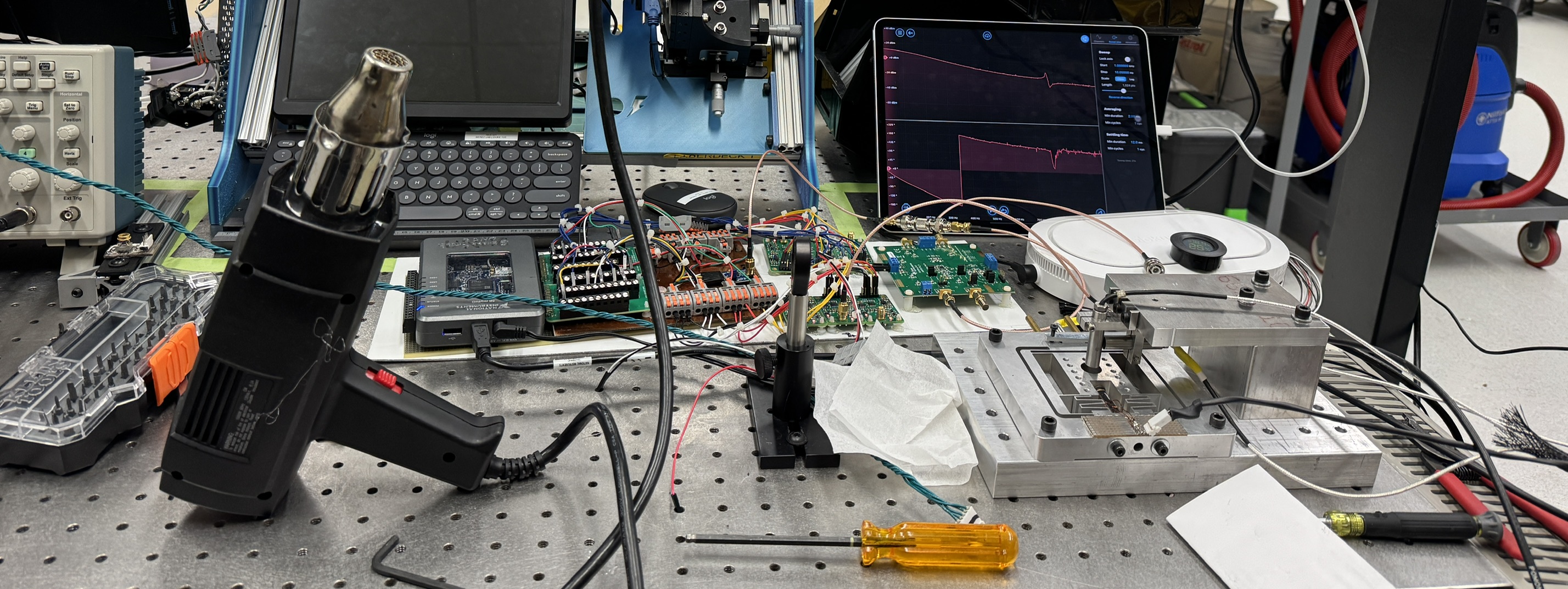
the next step going forward is to look at what affects these resonances. i tried blasting the system with a heat gun and suprisingly the resonant modes did not really change.
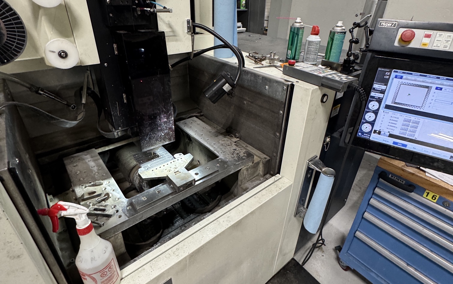
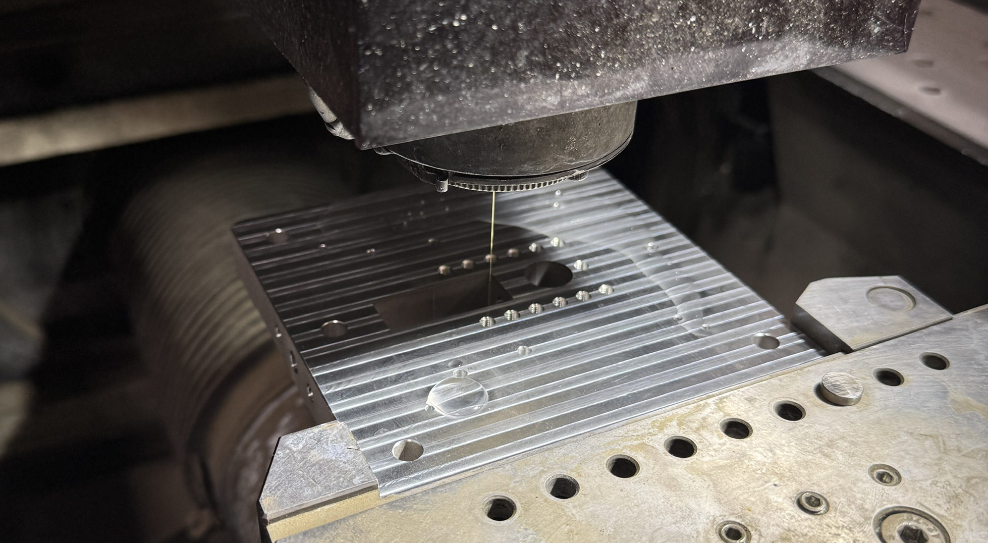
another testing route is to see how frame thickness affects these resonances. variants of the same flexure but with thicker frames were cut out as well.
this project is being handed off to a new team for 2026, so this is where my contributions end for now. I will likely continue working on optimizing the sensing for maximum speed and resolution.