automated high throughput laser focus mapping system

2025-11-16 · research

one thing people don't think about with metal 3D printers is that the laser isn't always focused where you'd expect it to be. the scan lens is supposed to put the focal point right on the build plane, but between optical aberrations, machine tolerances, calibration slop, and thermal drift, there can be real offset between where the beam actually focuses and where the powder is. even a couple millimeters of defocus changes the spot intensity enough to mess with melt pool depth, porosity, surface finish, etc. the most important thing to mitigate that is a direct result of a lower intensity spot is lack of fusion porosity. your part will look fine but have stress concentration heavy pores that are harder to detect. this could cause your hip implant or jet turbine blade to suddenly fail which is never a fun time.

current solutions on the market cost hundreds of thousands of dollars, and to commission the use of one usually costs around $50k per instance. the aim of this is to cut that down to around \$100 an instance in materials. the full system combines a low cost artifact-based approach with an automated sample processing machine.

relative power density for a single-mode gaussian beam can be represented as:

where \(z\) is the focus error and \(z_R\) is the rayleigh length. the result is a pretty gentle falloff if you're close, but once you get past maybe 30% of the rayleigh length the effect on spot intensity changes quite significantly. this offset varies spatially across the build plate, in a way that is not completely understood at any point in the process. you might be in perfect focus in the center and 3 mm off in the corners. and you'd never know unless you measured it.

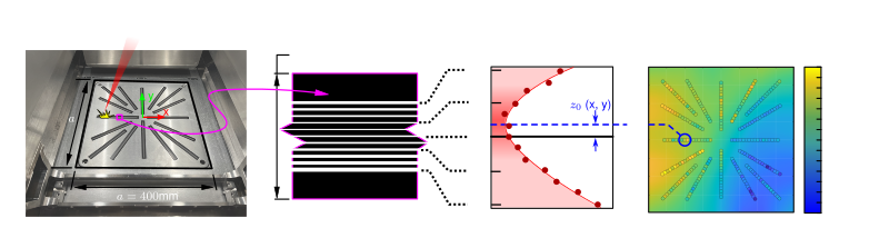
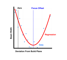
my advisor's earlier work (j. berez) showed you could figure out the focus offset at a given location by ablating tracks on anodized aluminum at a range of known z-offsets (by stepping the build platform up and down), measuring the track widths, and fitting the beam caustic to find where the minimum lands. the offset of that minimum from the build plane is the focus error. it worked, but it was manual, slow, and limited in how many points you could reasonably measure.

so this project was about doing that same idea but making it actually practical: more points, faster, less human effort. that meant redesigning the test artifact geometry, building a dedicated measurement device, and writing an image processing pipeline to automate the whole thing.

the artifacts

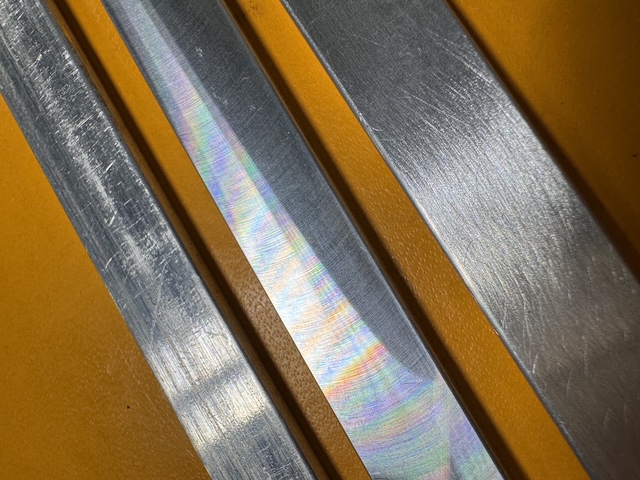
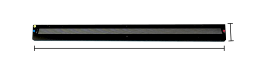
in order to capture the width of the laser beam at any point, a black anodized aluminum sample is used because the laser leaves behind a nice white on black pattern that is very condusive to imaging. the prior work used discrete rectangular coupons placed at cartesian grid positions on the build plate. I switched to a polar layout with long radial samples arranged like spokes across the build area, each one containing ablated tracks at programmed z-offsets spanning ±5 mm from the build plane. the nice thing about this geometry is that angular and radial resolution are decoupled. you get angular coverage from the number of spokes, and you can sample as finely as you want along the radial direction just by looking at more positions along each spoke's length. you don't have to go back and make more artifacts if you want higher spatial resolution, instead you can technically just take more images.

the measurement device

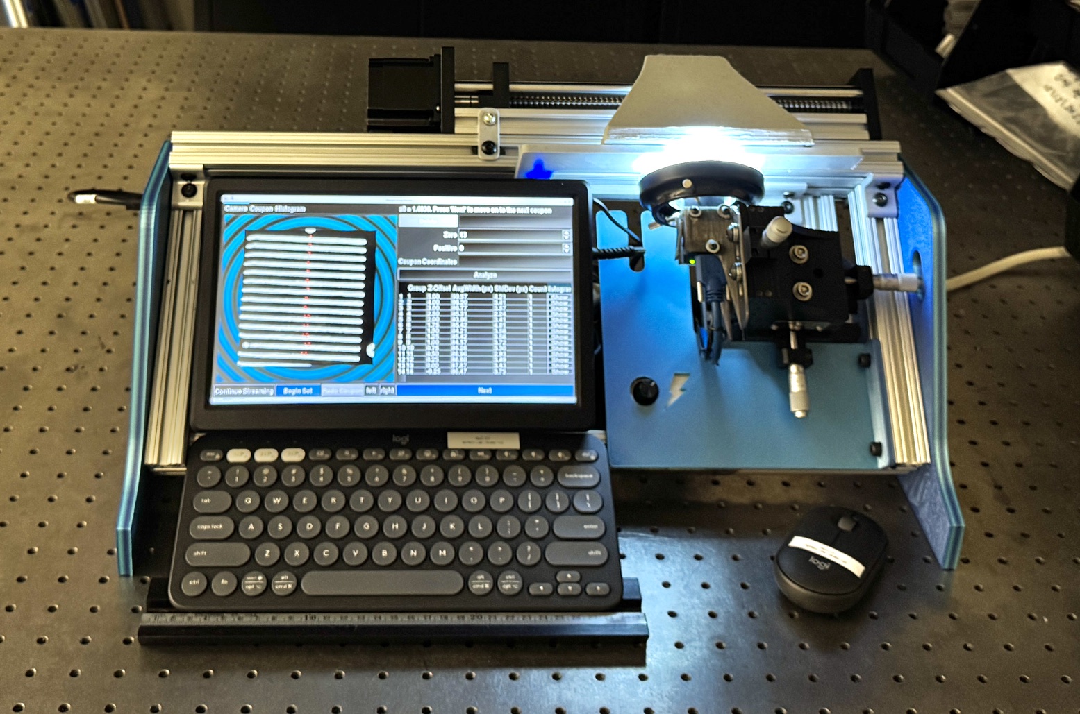
to actually image the ablated tracks I built a semi-inverted microscope setup. each artifact gets loaded face-down into the field of view of a monochrome 6K machine vision camera fitted with a 2× microscope objective. the usable field of view is about 4.4 mm × 4.4 mm, which is enough to see all the tracks at a single radial location. the camera sits on a 3-axis micrometer-driven translation stage for focusing and alignment, with a ring flash for illumination. a ball screw-driven motion stage translates each artifact laterally in controlled increments so I can step through the radial positions without touching anything.

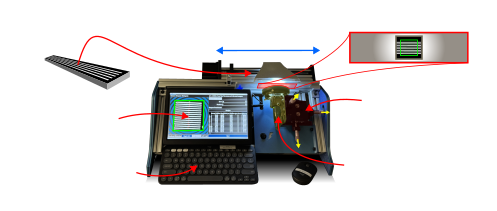
image processing

each captured frame goes through a pretty standard pipeline of gaussian smoothing (95×95 px kernel), otsu binarization, contour detection to isolate individual tracks. in order to measure tracks getting the orientation in frame is required for robustness in case of any misalignment. PCA on the filled contours gives you the track orientation, and then I cast rays perpendicular to that direction at evenly spaced locations along each track's length and measure the distance between the outermost contour intersections. that gives as many width samples per track as needed, I typically use something like 500-1000 points. to handle outliers such as track ends, breakages, and debris the mode of the width measurements are selected and anything outside of 2 standard deviations of that is removed. the average then comes from that cropped data.

finding focus offset

the beam caustic is modeled as:

where \(w_0\) is the minimum track width, \(z_0\) is the focus offset, and \(z_R\) is an effective rayleigh length. now, the ablated track width isn't the same thing as the beam's actual \(d_{4\sigma}\) width, the two are related through the material's ablation threshold and melt behavior. but the track-width profile is still symmetric about the focus plane, so fitting the caustic form still locates the minimum correctly. \(z_0\) comes out of the fit even though \(w_0\) and \(z_R\) are effective parameters rather than true beam parameters. all three get optimized simultaneously with a levenberg-marquardt solver.

results on an EOS M400

we ran this on an EOS M400-1 at oerlikon AM with a 400 mm x 400 mm build area and a 1000 W ytterbium fiber laser. tracks were ablated at 150 W and 2000 mm/s across ±5 mm of z-offset in 1 mm steps. 16 radial artifacts were measured at 14 positions each, with 4 repeats per position, giving 896 individual focus offset measurements.

the result was about ±2.5 mm of focus offset variation across the build area, with some non-averaged points hitting ±3 mm. repeatability was decent too, 90% of the measurement locations had a range of ≤0.33 mm across the four repeats.

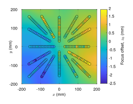
the tested machine has a rayleigh length of 4.79 mm per EOS service data. plugging that into the power density equation, ±2.5 mm of defocus means the laser is delivering up to ~21% less peak irradiance than it would at perfect focus, and the worst-case ±3 mm spots are losing ~28%. those offsets exceed what's been reported as the tolerance for acceptable melt pool penetration. the worst locations are above 50% of the rayleigh length, which is well past where you'd start to see real problems in parts.

this is on a production machine that was realistically calibrated. it's not broken, it just has the normal level of optical imperfection that comes with a big f-theta lens and a 400 mm scan field. most users would never know this variation existed without measuring it. maybe if you print a ton of parts and notice some weird variation in certain areas.

next steps are linking the measured focus offset to actual part outcomes, things like porosity and surface finish, and doing a proper uncertainty analysis to understand what's limiting the measurement precision.